Bell tests

The loophole free Bell experiments are among the top achievements in quantum information science over the last few years. However, as with other recent experimental validations of an a well accepted theory, the results did not change our view of reality. The few skeptics remained unconvinced, while the majority received further confirmation of a theory we already accepted. It turns out that this was not the case with the first Bell tests in the 1970s and 1980s (Clauser, Aspect etc. )

Jaynes, a prominent 20th century physicist who did some important work on light matter interaction did not believe that the electromagnetic field needs to be quantized (until Clauser’s experiment) and did extensive work on explaining optical phenomena without photons. As part of our recent work on modeling a quantum optics experiment using a modified version of classical electrodynamics (and no `photons’) we had a look at Jaynes’s last review of his neo-classical theory (1973). This work was incredibly impressive and fairly successful, but it was clear (to him at least) that it could not survive a violation of Bell’s inequalities. Jaynes’s review was written at the same time as the first Bell test experiments were reported by Clauser. In a show of extraordinary scientific honesty he wrote:

If it [Clauser’s experiment] survives that scrutiny, and if the experimental result is confirmed by others, then this will surely go down as one of the most incredible intellectual achievements in the history of science, and my own work will lie in ruins.

Three papers published

When it rains it pours. I had three papers published in the last week. One experimental paper and two papers about entanglement.

  1. Experimental violation of the Leggett–Garg inequality in a three-level system. A cool experimental project with IQC’s liquid state NMR group.    Check out the outreach article  about this experiment.
  2. Extrapolated quantum states, void states and a huge novel class of distillable entangled states. My first collaboration with Tal Mor and Michel Boyer and my first paper to appear in a bona fide CS journal (although the content is really mathematical physics). It took about 18 months to get the first referee reports.
  3. Entanglement and deterministic quantum computing with one qubit. This is a follow up to the paper above, although it appeared on arXiv  a few months earlier.

Nonlocal Measurements

My paper Nonlocal Measurements Via Quantum Erasure has  finally been published in PRL.  There is a short news story on the work on the IQC website. I also recently wrote a related blog post on nonlocal measurements for the IQC blog.

IQC blog post: Tomaytos, Tomahtos and Non-local Measurements


nl

Nonlocal measurements via quantum erasure, A. Brodutch and E. Cohen  Phys. Rev. Lett 116 (2016)


Misconceptions about weak measurements: 2. Weak, not noisy

It’s about time that I continue writing about misunderstandings surrounding weak measurements and weak values. This time I will try to explain the difference between weak measurements and noisy measurements.

Why weak? 

One of the first things we learn about quantum mechanics is that  the measurement process causes an unavoidable back-action on the measured system. As a consequence, some measurements are incompatible, i.e. the result of a measurement on observable  A  can change significantly if a different observable,  B, is measured before A.  A well known example is the measurements of position and momentum where the back-action leads to the Heisenberg uncertainty relation.

The measurement back-action can create  some seemingly paradoxical situations when we make counterfactual arguments such as

We measured A and got the result a, but had we measured B we would have go the result b which is incompatible with a.

These situations appear very often  when we consider  systems both past and future boundary conditions. In these cases they are known as pre and post selection (PPS) paradoxes. In PPS paradoxex the measurement back-action is important even when A and B commute.  An example is the three box paradox that I explain without mathematical detail:

A single particle is placed in one of three boxes A,B,C (actually in a superposition) at time t0 and is later found to be in some other superposition state at t1.  At time t0< t m < t1 one box is opened. The initial t0 and final t1 states of the particle are chosen in such a way that the following happens:

If box A is opened, the particle will be discovered with certainty. If box B is opened, the particle will also be found with certainty. If box C is opened the particle will be found with some probability. The situation seems paradoxical:

If the ball is found with certainty in box A, then it must have been in box A to begin with. But if it is also found with certainty in box B, so it must have been there …

One way to solve this apparent paradox is to note that the measurements are incompatible. i.e opening box A and not B,C is incompatible with opening box B and not A,C etc.

These are the types of questions that Aharonov Albert and Vaidman were investigating  1980s1 . Weak measurements were studied as a way to minimize the measurement back-action. These measurements then  provided a picture that arguably gives a solid (if somewhat strange) foundation to statements like the one above.

The motivation of weak measurements is therefore an attempt to derive a consistent picture where all observables are mutually compatible in a way which is similar to classical physics. In quantum mechanics this comes at a cost. The classical information gained by reading out the result of a single weak measurement is usually indistinguishable from noise. In other words  weak measurements are noisy measurements.


Weak, not noisy

Part of the confusion around weak measurements lies in the fact that the statement above is not a sufficient condition for a weak measurement. One may argue noise is not even a necessary requirement, it is rather, a consequence of quantum mechanics. Weak measurements may be noisy, but noisy measurements are, in most cases, not weak. To understand this fact it is good to examine  both a classical and quantum scenario.

The classical scenario

Walking on the beach you see a person drowning. Being  a good swimmer you go in and try to save this person. As you get back to the beach you see that he is not responsive and decide to to find if he is alive. You are now faced with the choice of how to perform the measurement.

A weak measurement – You try to get a pulse – The measurement is somewhat noisy since the pulse may be too weak to notice. It is also a weak measurement since it is unlikely to change this person’s state.

A noisy measurement – You start screaming for help. There is some small chance that the guy will wake up and tell you to shut up.

A noisy, strong measurement – You start kicking the guy in the head, hoping that he regains conciseness. This is a strong measurement, but it is also noisy. The person might be alive and you still won’t notice after kicking his head, moreover the kick in the head might kill him.

The quantum scenario

You want to find the \sigma_z component of a spin 1/2 particle.

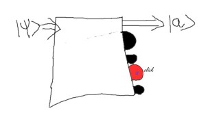
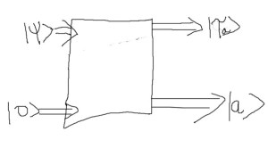
A weak measurement – Perform the usual von Neumann measurement with weak coupling. There is still some back-action but if the coupling is sufficiently weak you can ignore it. The down side is that you will get very little information.

A noisy measurement – Perform the weak measurement as above, but follow it with a unitary rotation and some dephasing.

A noisy, strong measurement – Perform a standard projective measurement, but then add extra noise at the readout stage. This could, for example,  be the result of a defective amplifier.

While all of the measurements above are noisy, only the weak measurements follow the original motivation of making a measurement with a weak back-action.

An extreme example

One neat example of a measurement which is noisy but not weak involves a wave function with a probability distribution that has no tails.

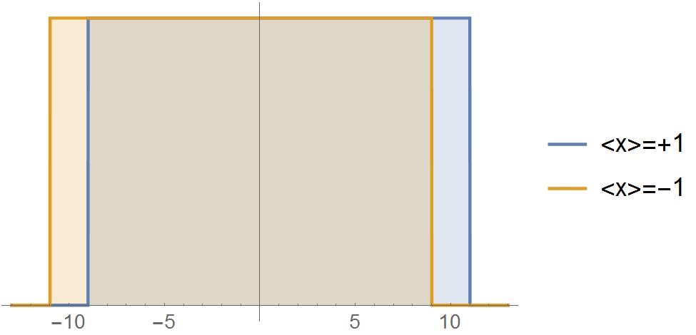
Take the measurement of a Pauli observable that has results \pm1 and imagine that after the readout we get the following probability distributions: If the system was initially in the state corresponding to +1 we get a flat distribution between -9 and 11, if the result is -1 we get a flat distribution between -11 and 9. The measurement is noisy, in fact any result between -9 and +9 will give us no information about the system. However it is not weak since any result outside this range will cause the state of the system to collapse into an eigenstate.

A pointer with no tails: The probability density function for the result of a  dichotomic measurement. A +1 state will produce the blue distribution while a   -1 state will produce the orange one. Although a result between -9 and +9 will provide no information, the measurement is still not weak.

It is not surprising that this type of measurement will not produce a weak value as the expectation value of a given set of measurements on a pre and post selected system.  While this is is obviously an extreme case,  any situation where the probability density function for the readout probabilities has no tails will not be weak for the same reason. The same is usually true in cases where the derivatives of the probability density function are very large. In less technical terms – noise is not a sufficient condition for a weak measurement.


1. To get a partial historic account of what AAV were thinking see David Albert’s remarks in Howard Wiseman’s QTWOIII talk on weak measurements (around minute 25-29) 


Misconceptions about weak measurements: 1. Weak ‘measurements’.

It seems that I am somehow drawn to controversial subjects. Maybe it’s my nature as an Israeli. Much of my Phd research has been around the controversial topic of ‘quantum discord‘.  Now I find myself working hard on the subject of my Master’s thesis, ‘weak measurements’, yet another topic which is both controversial and misunderstood.  Unlike quantum discord which became controversial mainly due to it’s popularity (aka the discord bubble),  weak measurements were controversial from day one.   This controversy  is, at leas in part, due to both misunderstandings, different interpretations, and choice of words; in particular the word `measurement’.

I first realized that the use of the word measurement may  cause of confusion after watching a recorded lecture by Anthony Leggett.  But the problem really sank in after many discussion with Marco Piani who helped me clarify my thoughts about the subject.  At one point Marco’s reaction reminded me of the phrase “You keep using that word. I do not think it means what you think it means.“.

Let me explain.

In a discussion of measurements, Asher Peres, one of the main critics of weak measurements (and my academic `grandfather’) wrote `The “detector clicks” are the only real thing we have to consider. Their observed relative frequencies are objective data.’ This is the usual sense we think of measurements in quantum information, a measurement  is a channel that takes a quantum state as input and gives probabilities (the relative frequencies) as an output.  Let us call this the quantum information approach. In more technical language a measurement is completely specified by the POVM elements. Roughly speaking any set of POVM elements that sum up to the identity can describe a measurement i.e probabilities for the various detectors clicking. However, a weak measurement cannot be described in this way, the POVM elements are at best, only part of the picture.


click

The quantum information approach. Quantum in – classical out


The first time I encountered the term POVM was during the time between my B.Sc and M.Sc when I started learning the basics of quantum information. As  an undergad, I was taught about a different type of quantum measurement. The quantum world, I was told, is made up of quantities that are observable; these correspond to Hermitian operators. The results of the measurements are eigenvalues and after the measurement the measured system will change its state to the relevant eigenvector, the so-called collapse of the wave function. I will call this the textbook approach. The big difference between this and the `quantum information approach’ (above) is that the channel has a classical input and a classical (eigenvalue) and quantum (eigenvector) output. This is closer in spirit to the `measurement’ in a weak measurement. However this framework does not have any variable strength.

TB

The textbook approach. Quantum in- classical [eigenvalue] and quantum [eigenvector] out.


The `textbook approach’ is unsatisfactory in two ways. First it allows a limited class of measurements that do not necessarily correspond to realistic situations. Second it does not include a dynamical picture: measurements simply happen. Although a full dynamical picture is still an (if not the) open problem, von Neumann gave the a reasonable dynamical picture for the measurement which is know as the von Neumann scheme. The measurement is described as a coherent interaction between the measured system and a (quantum) meter initially in a state |0>.  The interaction Hamiltonian is set up so that: if the system is in an eigenstate a of the desired observable, the meter will shift accordingly i.e it will end up in the state |a>.  Generally the system-meter state will be entangled after the measurement. With the right choice of interaction Hamiltonian the local picture will be  a mixed state that gives the right statistics for the textbook measurement. A slightly more elaborate picture can be used to describe more general measurements.

vN

The von Neumann scheme. Quantum [product system-meter] in- quantum [entangled system-meter] out.


A weak measurement is a measurement in this sense, i.e it is a channel that has a system-meter (quantum) input and a system-meter (quantum) output. The measurement can be followed by a readout stage where a single detector `clicks’, but this part simply tells us something about the meter and only indirectly about the system whose state has changed.To complete the transition from the von Neumann scheme to a weak measurement we simply need to make the interaction Hamiltonian weak. It should be so weak that, after the measurement, the shifts corresponding to different eigenvalues will strongly overlap. The first  advantage of this  method is that the system state is virtually unchanged by the measurement process. Other, surprising  advantages follow, especially when one considers the fact that this measurement process is symmetric with respect to time.

I hope I convinced you that the term `measurement’ means different things to different people; While quantum information theorists say measurement and mean `a quantum to classical channel’ the weak measurement community think of a `quantum to quantum channel’. I believe this is major source of confusion that leads to controversy around weak measurements. My advice to people in the quantum information community is: either stop thinking about weak measurements as measurements, or read the literature and try to convince yourself that this channel represents the closest thing we have to a measurement in quantum theory.  Either way stop trying to understand weak measurements simply in terms of POVM elements.


In upcoming posts I will try to clarify some other misconceptions including the difference between `noisy measurements’ and `weak measurements’, and an explanation of what is anomalous about ‘anomalous weak values’.

Discord and completely positive maps

After over two years of work  we finally published our results showing that the connection between discord and complete positivity is quite weak, and probably has no operational significance. But let me start at the beginning:

In the beginning… and then there was a big discussion/argument about possible maps describing the evolution of a quantum system interacting with the environment. In the case where they are initially correlated this discussion is still not settled. In 2007 came a paper by Cesar Rodriguez-Rosario Kavan Modi, Aik-meng Kuah, Anil Shaji and ECG Sudarshan titled “Completely positive maps and classical correlations“, I call it Cesar and Kavan’s paper. They examined a situation where some initial family of system-environement, $$mathcal{SE}$$ states is classically correlated (has zero discord). It turns out that such a family of states is in the consistency domain of  a completely positive assignment map. In slightly less technical language: given a family of classically correlated $$mathcal{SE}$$ states it is possible to describe the evolution of the system using a completely positive map. Without going into details this comes with some caveats. Cesar, Kavan and Alán Aspuru-Guzik explained these caveats in another paper.

About a year after Cesar and Kavan’s paper Alireza Shabani and Daniel Lidar published a paper titled “Vanishing Quantum Discord is Necessary and Sufficient for Completely Positive Maps” This result was published in PRL, I will call it the SL paper. It made a lot of waves and has since been cited around 150 times. Unfortunately no one really understands it. I don’t know who should be blamed here, the authors for writing an unreadable paper (I assume they can read it), the editor for accepting an unreadable paper, or the referees who thought the paper was readable. But as it stands this paper was accepted, and since it was published in a prestigious journal and has such a bombastic title, people love to cite it. Especially to justify their research on discord. I guess I could start a rant but it’s nothing new so let us return to the story.

In September 2010 I had the extreme pleasure of attending the “Quantum Coherenece and Decoherence” workshop in Benasque where I met Cesar and Animesh Datta. After a short conversation about discord and interesting results in the field we discovered that although we have all cited SL we don’t know what they actually claim. We all assumed it was the “necessary” part of Cesar and Kavan’s “sufficient” result for completely positive maps but none of us could really explain the bottom line. After spending a few days in trying to understand the paper together we finally gave up, and instead came up with a counterexample. That is, we found a family of discordant states which is consistent with a completely positive assignment map.

A few weeks later I met Kavan in Singapore and we discussed this result further…

[missing reel]

.. and finally  Ángel Rivas joined our jolly group. The work was very slow, mostly due to us being on 4 different continents. By the time time I was at IQC we had a draft. When Kavan came to visit we finalized the paper.

The final version is much more then a comment on SL’s result. We showed that the problem of finding the map that correctly describes the evolution is a matter of how the problem is stated. More to the point, we showed that in at least thee sensible frameworks for approaching this problem there is at best a one way connection between positivity of the map and discord. Presumably there might be a framework where zero discord is both necressary and sufficient for completely positive maps. Unfortunately we were unable to identify this framework.


Vanishing quantum discord is not necessary for completely-positive maps
Aharon Brodutch, Animesh Datta, Kavan Modi, Ángel Rivas, César A. Rodríguez-Rosario arXiv:1212.4387Phys. Rev. A 87, 042301


Quantum discord

After a long an eventful month that included a visit by Kavan Modi to IQC and my visit to Israel (I’m posting from Israel), it’s time I got back to writing something. This time I’ll say something about my work for the past four years (as promised). One of the main subjects of my research is quantum correlations, and their role in defining the difference between quantum and classical (not quantum) systems.
Imagine a piece of information shared between two people Alice and Bob. Now think of a way to quantify the correlations between them. One way to quantify correlations is to ask what can Alice know about Bob’s part of the information by looking at her own part.
For example lets say Alice and Bob are each given a queen from a chess board. Alice then looks at her queen and sees it is white. She now knows Bob’s queen must be black. Alice and Bob are strongly correlated, since Alice always knows Bob’s piece by looking at her own.
For the second example Alice and Bob are each given a queen, but this time from a Deck of cards. If Alice sees a red queen she can say that it is more likely that Bob has a black queen, but she has no certainty. Correlations are lower in this case then in the chess example.
There is another way to account for correlations. We can ask about difference between the information in Alice and Bob’s hands individually and the information in their hands together. In the chess example Alice and Bob can each get one of two types of queens: black or white Together they also have two options Black White or White Black.
It turns out that both options for quantifying correlations are the same. To see this in the example we need to quantify the information in bits. Since Bob has two options in his hand “black queen” or “white queen” he has one bit of information. The amount of information Alice can discover about Bob is precisely this one bit. So they have one bit of correlations. Alternatively we can say that Alice has one bit of information: “black queen” or “white queen”; Bob has one bit of information: “black queen” or “white queen” and together they also have one bit “black white” or “white black”. The difference (1+1)-1 is again 1 bit so there is one bit of correlations.
Since i’m avoiding maths you will have to take my word that both methods give the same result in all cases… in the classical world. In the quantum world things are a bit different.
There are two essential (and related) aspects of quantum theory that make these two ideas about how to to quantify correlations give different results. 1) Measurements affect the system. If Alice wants to know the color of her queen, she needs to make a measurement, this measurement can change the state of the system; and 2) Quantum systems can be correlated in a much stronger way then classical systems, a phenomenon known as entanglement.
Before discussing the first aspect in detail, I will say a bit about entanglement. Entanglement was a term coined by Schrodinger in his famous “cat” paper, this paper was inspired by the earlier “paradox” of Einstein Podolski and Rosen (EPR). They showed that quantum mechanics predicts a situation where a system shared by two parties is in a well defined state although locally it is not defined. A system is in a well defined state if making a measurement on this system will give some result with certainty. So if I give Alice and Bob an entangled system I can predict the result of a measurement made on the whole system, but I cannot predict the result of a measurement made by Alice and Bob separately.
Entanglement is the most remarkable prediction of quantum mechanics, and in one way of another it is the driving force behind most of the really cool quantum phenomena. From quantum computers to Schrodinger’s cat. Nevertheless entanglement does not account for all the non-classical features of the theory. At least not directly. When discussing correlations, measurements and their effects on the system play a crucial role in describing non-classicality. To explain quantum measurements we can imagine a quantum system as an arrow pointing to some direction, X, in the simplest case we can think of this problem in two dimensions.
A quantum measurement is a question regarding the direction of the arrow. Is the arrow pointing in direction A? This has one of two results either yes or no. The probability is given by the angle between the “actual” direction and the direction in question. The effect of the measurement is that the arrow will now point in the same direction as the result. If the answer is yes it will point in direction A if the answer is no, it will point in the opposite direction.


A quantum measurement will "collapse" the state X into A or Not A.

A quantum measurement will “collapse” the state X into A or Not A.

Ok so what does this have to do with correlations? Well lets go back to the two definitions for correlations. The first was “What information can Alice find about Bob by looking at her own system”. In the quantum case this is no a clear question, we need to also say what measurement Alice is making. Different measurements will reveal different information about Bob. The second definition for correlations is what is the difference between the information in Alice’s hands plus the information in Bob’s hands and the information in their joint system” This is not directly related to measurement, so clearly it is not the same as the first definition. The difference between these definitions in the quantum case is the quantum discord. It is a measure of the “quantumness” of correlations.
As it turns out discord can be found in many interesting quantum systems and paradigms, but it is not yet clear what this means…

I’m an expert

Two expected, but long awaited events happened on my birthday. One: I found out that my Phd was approved, so no more bureaucratic shit regarding that. Two: The review paper on discord and similar quantities was finally published. This sums up about one and a half years’ work spent on reading, writing and rewriting this review with my collaborators.  Two versions have been posted on  arXiv  since the end of last year. The latest one, posted in August, is pretty much the published version.

I will soon post something longer about discord and non-classical correlations, for now it is enough to say that quantum theory allows more general correlations then a classical theory.  Entanglement is the best example of these types of correlations, but as it turns out there are unentangled systems with non-classical correlations. Quantum discord captures entanglement and more (but not everything).

Since the beginning of the century (i.e 12 years ago) people started studying these kinds of correlations “beyond” entanglement in various forms and physical scenarios. The area exploded about 5 years ago and discord became a “hot” topic. The review includes almost all the work done on the subject until the end of 2011. discord was studied in so many different scenarios like quantum information, thermodynamics, many body systems, relativistic quantum information and others which made work on this review so much fun, on the one hand, but a lot of work on the other.


Faster than light quantum information

A cool new paper appeared in Nature Physics this week and made a lot of waves (at least on my facebook feed).

In this paper titled “Quantum non-locality based on finite-speed causal influences leads to superluminal signalling” the authors show a method for testing if the “weird” effects of entanglement such as the violation of Bell inequalities can be explained using a faster then light source for exchanging information.

The main problem with these kinds of theories is that the usual Bell experiments can at best put a lower bound on the speed of exchanging this kind of information. The way to overcome this problem is to look at Bell violations in a 4 party system. The result of the paper is that one can perform a test that requires the speed of these causal influences to be infinite.

http://www.nature.com/nphys/journal/vaop/ncurrent/full/nphys2460.html