Scaling up

It’s been a while since I last wrote here, meanwhile a lot has happened. On a global scale we’re going through a pandemic, on a personal level, I’ve left academia to start a quantum computing company.

A while ago I heard Carl Caves say something like “You should work on what you consider to be the most important problem in physics”. Most important is of course subjective. To me it has always been about understanding and pushing the limits of quantum mechanics while trying to stay within the realm of what we can actually test in experiment. Large quantum computers would open a new realm of science, pushing quantum theory far beyond anything that nature can demonstrate. And so, building these machines and scaling them up is certainly the most exciting science we can do today.

Ok, but we already know that…

I have to be realistic, building a quantum computer is really hard, also there are many good people doing that, so where can I contribute? This was the question my co-founders and I were asking ourselves about a year ago. Before giving my answer I want to first define the goal: building a large quantum computer.

But what is large?

Going back to the original goal, I would like to see a machine that could potentially demonstrate radically new physics. But that’s difficult to define, perhaps we would know it when we see it, but where can we aim that’s more concrete?

Since we are talking about a computer, what we want is machines that perform computations which are essentially impossible on a classical computer (AKA quantum supremacy). It’s a good first step but it’s not good enough. There are many things in nature that cannot be simulated on classical computers. One can make the point that quantum supremacy does not offer anything more interesting than a chemical reaction in terms of its ability to demonstrate radically new physics. What we need is some additional criteria which is difficult to define precisely but would ultimately mean one of two things:

  • Using quantum computers to answer questions that cannot be answered in a lab.
  • Using quantum computers to search for violations of known physics.

We are still (in my opinion) many years away from taking either of these seriously, however we are near the stage where quantum computers can become useful scientific tools that can at the very least be more efficient than some experiments in terms of manpower, money and time. To me, that is the real first step in building machines that would eventually open a new realm of science and technology. I am optimistic that this first step would also open the door for other use cases and I believe that we are close.

Building quantum computers

There are generally two main ways to improve the performance of a quantum computer. Increase the number of qubits and improve the control over these qubits. The problem is that it’s difficult to do both, in fact, more qubits means more control issues, and it’s difficult to decide which is more important. The obvious solution is to focus on small high-quality devices and then interconnect them. This of-course comes with two difficulties, building the interconnects and dealing with connectivity issues. That’s where Entangled Networks comes in.

We decided that since the most important problem is scaling quantum computers, we should focus on the best solution, interconnecting small high-quality processors. It’s an exciting problem and one that needs to be solved as soon as possible in order to build quantum computers that would be of interest to the general community. It is also a problem that can be solved within a reasonable time-frame. I am happy to report that we are making good progress. On the personal level it’s a great ride with many ups and downs (as expected), new challenges, and lots of fun.

The mathematical foundations of quantum mechanics

Von Neumann’s 1932 book “The mathematical foundations of quantum mechanics” was a cornerstone for the development of quantum theory, yet his insights have been mostly ignored by physicists. Many of us know that the book exists and that it formalizes the mathematics of operators on a Hilbert space as the basic language of quantum theory, but few have bothered to read it; feeling that as long as the foundations are there, we don’t need to examine them. One reason the book has never been popular as a textbook is that von Neumann does not Dirac’s notation. He admits that Dirac’s representation of quantum mechanics is “scarcely to be surpassed in brevity and elegance” but then goes on to criticize its mathematical rigor, leaving us with a mathematically rigorous treatment but a notation that is difficult to follow and a book that nobody ever reads.

Today, von Neumann’s book is brought up often in connection with foundations research, which is perhaps not surprising given the author’s original intent as stated in the preface:

the principle emphasis shell be placed on the general and fundamental questions which have arisen in connection with this theory. In particular , the difficult problems of interpretation, many of which are even now not fully resolved, will be investigated in detail.

Two particular results are often cited

  1. Von Neumann’s (presumably incorrect) proof of impossibility for a hidden variable model of quantum theory.
  2. The von Neumann measurement scheme, which is the standard formalism for describing a quantum measurement.

The description of the measurement scheme is (or at least was to me) a little surprising. The usual textbook description of von Neumann’s work is to start with the Hamiltonian that couples the measurement device to the system under measurement, and to show that it produces the right dynamics (up to the necessity for state collapse). It turns out that von Neumann’s motivation was in some sense the opposite.

He begins by considering a classical measurement and showing that the observer must be external to the measurement, i.e there are three distinct objects, the system under observation, the measurement device, and the observer. Keeping this as a guide, von Neumann provides a dynamical process where the observer is not quantum mechanical while the measurement device is. The important point is that the precise cut between the (classical) observer and the (quantum) measurement device, is not relevant to the physics of the system, just as in classical physics.

Von Neumann does not suggest that he solves the measurement problem, but he does make it clear that the problem can be pushed as far back as we want, making it irrelevant for most practical purposes, and in some ways just as problematic as it would be in classical physics. Many of us know the mathematics, and could re-derive the result, but few appreciate von Neumann’s motivation: understanding the role of the observer.

Beyond classical (but is it quantum?)

The accepted version of “Interpreting weak value amplification with a toy realist model” is now available online. The work was an interesting exercise involving two topics in the foundations of physics: Weak values and stochastic electrodynamics. Basically we showed that a recent quantum optics experiment from our lab could be re-interpreted with a slightly modified version of classical electrodynamics.

The aim of the work was to develop some intuition on what weak values could mean in a realist model (i.e. one where the mathematical objects represent real “stuff”, like an electromagnetic field). To do this we added a fluctuating vacuum to classical electrodynamics. This framework (at least at the level we developed it) does not capture all quantum phenomena, and so it is not to be taken seriously beyond the regime of the paper, but it did allow us to examine some neat features of weak values and the experiment.

One interesting result was the regime where the model succeeds in reproducing the theoretical results (the experimental results all fall within this regime), which provided insight into weak values. Specifically, the model works only when the fluctuations are relatively small. Going back to the real world, this provide new intuition on the relation between weak values and the weak measurement process.

The experiment we looked at was done in Aephraim Steinberg‘s light matter interaction lab by Matin Hallaji et al. a few months before I joined the group. It was a ‘typical’ weak value amplification experiment with a twist. In an idealized version, a single photon should be sent into an almost balanced Mach Zehnder interferometer with a weak photon counting (or intensity) measurement apparatus on one arm (see figure below). The measurement is weak in the sense that it is almost non-disturbing, but also very imprecise, so the experiment must be repeated many times to get a good result. So far nothing surprising can happen, and we expect to get a result of 1/2 photon (on average) going through the top arm of the interferometer. To get the weak value amplification effect, we post-select only on (those rare) events where a photon is detected at the dark port of the interferometer. In such a case, the mean count on the detector can correspond to an arbitrarily large (or small, or even negative) number of photons.

The twist with the experiment was to use a second light beam for the photon counting measurement. This was the first time this type of weak measurement was done in this way, and is of particular importance since many of the previous experiments could be explained using standard electrodynamics. In this case, the photon-photon interaction is a purely quantum effect.

In reality the experiment described above was not feasible due to various imperfections that could not avoided, so a compromise was made. Instead of sending a single photon, they used a coherent beam with around 10-100 photons. To get the amplification effect on a single photon, they used a trick that would increase the number of photons by 1 and only looked for the change in the signal due to the extra photon. The results showed that the same amplification as the ideal case. However, there remained (and still remains) a question of what that amplification means. Can we really talk about additional photons appearing in the experiment?

As we showed, the results of the experiment can be explained (or at least reproduced) in a model which is more intuitive than quantum theory. Within that model it is clear that the amplification is a real, i.e the post-selected events corresponded to cases where more light traveled through the top arm of the interferometer.

The model was based on classical electrodynamics with a slight modification, we assumed that fields fluctuated like the quantum vacuuum. This turned out to be sufficient to get the same predictions as quantum theory in the regime of the experiment. However, we showed that this model would not work if the intensity of the incoming light was sufficiently small, and in particular it would not work for something like a single photon.

Our model has a clear ‘reality’, i.e the real field is a fluctuating classical EM field, and so it provides a nice start for a more general theory that has weak values as its underlying real quantities. One important feature of the model is the regime where it makes accurate predictions. It turns out that there are two bounds on the regime of validity. The first is a requirement that the light is coherent and is not too weak, this roughly corresponds to being in a semi-classical regime. The second is that the probability of detecting photons at the dark port is not significantly effected by the fluctuation which is similar to the standard weak measurement requirement, i.e. that the measurement back-action is small.

My main takeaway from the work was that the weak values ended up being the most accurate experimentally accessible quantity for measuring the underlying field. Making a leap into quantum theory, we might say that weak measurements give a more accurate description of reality than the usual strong measurement.

The result also set a new challenge for us: Can we repeat the experiment in the regime where the model brakes down (e.g. with single photons)?

Bell tests

The loophole free Bell experiments are among the top achievements in quantum information science over the last few years. However, as with other recent experimental validations of an a well accepted theory, the results did not change our view of reality. The few skeptics remained unconvinced, while the majority received further confirmation of a theory we already accepted. It turns out that this was not the case with the first Bell tests in the 1970s and 1980s (Clauser, Aspect etc. )

Jaynes, a prominent 20th century physicist who did some important work on light matter interaction did not believe that the electromagnetic field needs to be quantized (until Clauser’s experiment) and did extensive work on explaining optical phenomena without photons. As part of our recent work on modeling a quantum optics experiment using a modified version of classical electrodynamics (and no `photons’) we had a look at Jaynes’s last review of his neo-classical theory (1973). This work was incredibly impressive and fairly successful, but it was clear (to him at least) that it could not survive a violation of Bell’s inequalities. Jaynes’s review was written at the same time as the first Bell test experiments were reported by Clauser. In a show of extraordinary scientific honesty he wrote:

If it [Clauser’s experiment] survives that scrutiny, and if the experimental result is confirmed by others, then this will surely go down as one of the most incredible intellectual achievements in the history of science, and my own work will lie in ruins.

Updates

Some updates from the past 10 months…

  1. Papers published
  2. Preprint: Weak values and neoclassical realism
    My first paper with the Steinberg group is hardcore foundations.  Not only do we use the word ontology throughout the manuscript, we analyse an experiment using a theory which we know is not physical. Still, we get some nice insights about weak values.

Going integrated

As a quantum information theorist, the cleanest types of results I can get are proofs that something is possible, impossible or optimal. Much of my work focused on these types of results in the context of measurements and non-locality. As a physicist, it is always nice to bring these conceptual ideas closer to the lab, so I try to collaborate with experimentalists. The types of problems an experimental group can work on are constrained by technical capabilities. In the case of Amr Helmy’s group, they specialize in integrated photonic sources so I now know something about integrated optics.

When I started learning about the possibilities and constraints in the group, I realized that the types of devices they can fabricate are much better suited for work in continuous variables as opposed to single photons. I also realized that no one explored the limitations of these types of devices. In other words, we did not know the subset of states that we could generate in principle (in an ideal device).

In trying to answer this question we figured out that, with our capabilities,  it is in principle (i.e in the absence of loss) possible to fabricate a device that can generate any Gaussian state (up to some limitations on squeezing and displacement). What turns out to be even nicer is that we could have a single device that can be programmed to generate any N-mode Gausssian state. The basic design for this device was recently posted on arXiv.
Fig4_Page_1

We left the results fairly generic so that they could be applied to a variety of integrated devices, using various semiconductors. The next step would be to apply them to something more specific and start accounting for loss and other imperfections. Once we figure that out, we (i.e. the fab guys) an go on to building an actual device that could be tested in the lab.

Dynamically Reconfigurable Sources for Arbitrary Gaussian States in Integrated Photonics Circuits A. Brodutch Ryan Marchildon and Amr Helmy arXiv:1712.04105

Tomaytos, Tomahtos and Non-local Measurements

In the interest of keeping this blog active, i’m recycling one of my old IQC blog posts

One of my discoveries as a physicist was that, despite all attempts at clarity, we still have different meanings for the same words and use different words to refer the the same thing. When Alice says measurement, Bob hears a `quantum to classical channel’, but Alice, a hard-core Everettian, does not even believe such channels exist. When Charlie says non-local, he means Bell non-local, but string theorist Dan starts lecturing him about non-local Lagrangian terms and violations of causality. And when I say non-local measurements, you hear #$%^ ?e#&*?.  Let me give you a hint, I do not mean ‘Bell non-local quantum to classical channels’, to be honest, I am not even sure what that would mean.

So what do I mean when I say measurement? A measurement is a quantum operation that takes a quantum state as its input and spits out a quantum state and a classical result as an output (no, I am not an Everettian). For simplicity I will concentrate of a special case of this operation, a projective measurement of an observable A. The classical result of a projective measurement is an eigenvalue of A, but what is the outgoing state?

textbookM

A textbook (projective) measurement.  A Quantum state |\psi\rangle  
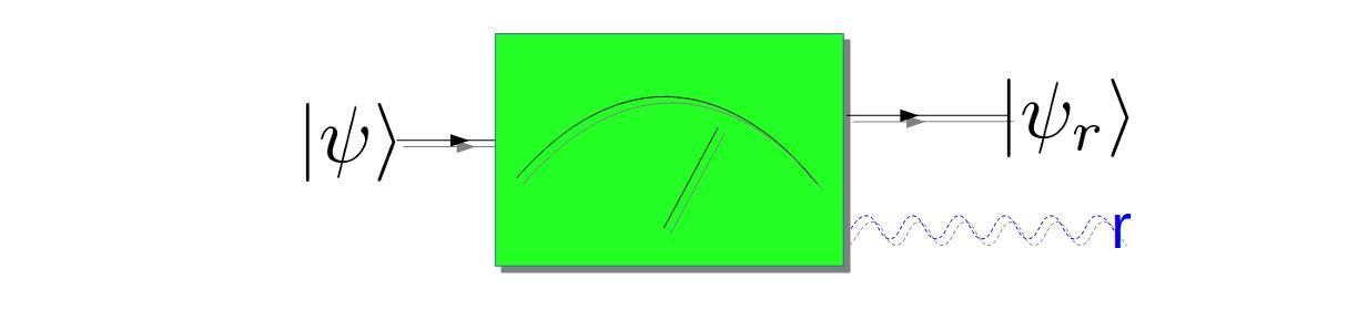
goes in and a classical outcome “r” comes out together with a corresponding  quantum state |\psi_r\rangle.

The Lüders measurement

Even the term projective measurement can lead to confusion, and indeed in the early days of quantum mechanics it did. When von Neumann wrote down the mathematical formalism for quantum measurements, he missed an important detail about degenerate observables (i.e Hermitian operators with a degenerate eigenvalue spectrum). In the usual projective measurement, the state of the system after the measurement is uniquely determined by the classical result (an eigenvalue of the observable). Consequently,  if we don’t look at the classical result, the quantum channel is a standard dephasing channel. In the case of a degenerate observable, the same eigenvalue corresponds to two or more orthogonal eigenstates. Seemingly the state of the system should correspond to one of those eigenstates, and the channel is a standard dephasing channel. But a degenerate spectrum means that the set of orthogonal eigenvectors is not unique, instead each eigenvalue has a corresponding subspace of eigenvectors. What Lüders suggested is that the dephasing channel does nothing within these subspaces.


Example

Consider the two qubit observable A=|00\rangle\langle 00 |. It has eigenvalues 1,0,0,0. A  1 result in this measurement corresponds to “The system is in the state |00\rangle “.  Following a measurement with outcome 1 , the outgoing state will be |00\rangle . Similarly, a 0 result corresponds to “The system is not in the state |00\rangle “. But here is where the Lüders rule kicks in. Given a generic input state \alpha|00\rangle+\beta|01\rangle+\gamma|{10}\rangle+\delta|{11}\rangle   and a Lüders measurement of A with outcome 0, the outgoing state will be  \frac{1}{\sqrt{|\alpha|^2+|\beta|^2+|\gamma|^2}}\left[\beta|{01}\rangle+\gamma|{10}\rangle+\delta|{11}\rangle\right].


Non-local measurements

The relation to non-locality may already be apparent from the example, but let me start with some definitions. A system can be called non-local if it has parts in different locations, e.g. one part on Earth and the other on the moon. A measurement is non-local if it reveals something about a non-local system as a whole. In principle these definitions apply to classical and quantum systems. Classically a non-local measurement is trivial, there is no conceptual reason why we can’t just measure at each location. For a quantum system the situation is different. Let us use the example above, but now consider the situation where the two qubits are in separate locations. Local measurements of  \sigma_z will produce the desired measurement statistics (after coarse graining) but reveal too much information and dephase the state completely, while a Lüders measurement should not. What is quite neat about this example is that the Lüders measurement of |{00}\rangle cannot be implemented without entanglement (or quantum communication) resources and two-way classical communication. To prove that entanglement is necessary, it is enough to give an example where entanglement is created during the measurement. To show that communication is necessary, it is enough to show that the measurement (even if the outcome is unknown) can be used to transmit information. The detailed proof is left as an exercise to the reader. The lazy reader can find it here (see appendix A).

This is a slighly modified version of a  Feb 2016 IQC blog post.  

Three papers published

When it rains it pours. I had three papers published in the last week. One experimental paper and two papers about entanglement.

  1. Experimental violation of the Leggett–Garg inequality in a three-level system. A cool experimental project with IQC’s liquid state NMR group.    Check out the outreach article  about this experiment.
  2. Extrapolated quantum states, void states and a huge novel class of distillable entangled states. My first collaboration with Tal Mor and Michel Boyer and my first paper to appear in a bona fide CS journal (although the content is really mathematical physics). It took about 18 months to get the first referee reports.
  3. Entanglement and deterministic quantum computing with one qubit. This is a follow up to the paper above, although it appeared on arXiv  a few months earlier.

Towards quantum supremacy

 Quantum phenomena do not occur in a Hilbert space. They occur in a laboratory.

Asher Peres

Being a theorist, it is easy to forget that physics is an empirical science.  This is especially true for those of us working on quantum information. Quantum theory has been so thoroughly tested, that we have gotten into the habit of assuming our theoretical predictions must correspond to physical reality. If an experiment deviates from the theory, we look for technical flaws (and usually find them) before seeking an explanation outside the standard theory. Luckily, we have experimentalists who insist on testing our prediction.

Quantum computers are an extreme prediction of quantum theory. Those of us who expect to see working quantum computers at some point in the future, expect the theory to hold for fairly large systems undergoing complex dynamics.  This is a reasonable expectation but it is not trivial.  Our only way to convince ourselves that quantum theory holds at fairly large scales, is through experiment. Conversely, the most reasonable way to convince ourselves that the theory breaks down at some scale, is through experiment. Either way, the consequences are immense,  either we build quantum computers or we make the most significant scientific discovery in decades.

Unfortunately, building quantum computers is very difficult.

There are many different routes towards  quantum computers.  The long and difficult roads, are those gearing towards universal quantum computers, i.e those that are at least as powerful as any other quantum  computer. The (hopefully) shorter and less difficult roads are those aimed at specialized (or semi or sub-universal) quantum computers. These should outperform classical computers for some specialized tasks and allow a demonstration of quantum supremacy; empirical evidence that quantum mechanics does not break down at a fairly high level of complexity.

One of the difficulties in building quantum computers is optimizing the control sequences. In many cases we end up dealing with catch-22. In order to optimize the sequence we need to simulate the system; in order to simulate the system we need a quantum computer; in order to build a quantum computer we need to optimize the control sequence…..

Recently Jun Li and collaborators found a loophole. The optimization algorithm requires a simulation of the quantum system under the imperfect pulses. This type of simulation can be done efficiently on the same quantum processor. We can generate the imperfect pulse `perfectly’, on our processor and it can obviously simulate itself.   In-fact, the task of optimizing pulses seems like a perfect candidate for demonstrating quantum supremacy.

I was lucky to be in the right place at the right time and be part of the group that implemented this idea on a 12-qubit processor. We showed that at the 12-qubit level, this method can outperform a fairly standard computer. It is not a demonstration of quantum supremacy yet, but it seems like a promising road towards this task. It is also a promising way to optimize control pulses.

As a theorist, I cannot see a good reason why quantum computers will not be a reality, but it is always nice to know that physical reality matches my expectations at least at the 12-qubit level.

P.S – A similar paper appeared on arXiv a few days after ours.

  1. Towards quantum supremacy: enhancing quantum control by bootstrapping a quantum processor – arXiv:1701.01198
  2. In situ upgrade of quantum simulators to universal computers – arXiv:1701.01723
  3. Realization of a Quantum Simulator Based Oracle Machine for Solving Quantum Optimal Control Problem – arXiv:1608.00677

Entangled cats and quantum discord

It turns out that few people appreciate the relation between Schrödinger’s cat and entanglement.  When we hear entanglement, the first paper that comes to mind is Einstein Podolsky and Rosen’s “Can Quantum-Mechanical Description of Physical Reality Be Considered Complete?”  EPR were the first to point out a strange prediction of quantum mechanics (which we now call entanglement),  but the   term entanglement (or its German equivalent) was coined by Schrödinger in a  paper  inspired by EPR. In the same paper Schrödinger describes an experiment involving a cat interacting with a  “small flask of hydrocyanic acid” (and a Geiger counter etc.) such that, at some point the best quantum description of the cat-flask system is an entangled state. If one then ignores the state of the flask, the cat is in a mixture of being dead and alive (and not in a superposition as some wold have you believe). Schrödinger noted that this is a peculiar situation,  the cat’s state has large uncertainty (it is maximally mixed) while the cat+flask etc. are in a well defined state, that is, the uncertainty is at the minimum allowed by the theory. We call such a state a pure state.

Schrödinger coined the term entanglement in the context of pure quantum states. A pure quantum state describing two subsystems is entangled  if (and only if) the state of each subsystem is mixed, i.e (within the context of the relevant operators) there is no (rank 1) measurement that yields a definite outcome1.  But in reality the states we encounter are mixed and Schrödinger’s definition cannot be applied in a straightforward way.

A mixed quantum state is similar to a composite color such as pink, brown or white which have no specific wavelength.  Any composite color can be made by mixing elements from a set of primary colors such as red green and blue (RBG) but one can choose different conventions to produce the same color2. Similarly, a mixed quantum state does not have a unique decomposition in terms of pure quantum states.  The cat in the box is in a mixture of being dead and alive, yet it is also in a mixture of being in various superpositions of dead and alive.  It turns out that this creates a serious problem when we try to define mixed state entanglement.

The standard way to define entanglement is to look for a decomposition into pure non-entangled states. So, if we can find some way to describe the mixed quantum state as a mixture of non-entangled (i.e separable) states, then the state is separable.  This is a convenient mathematical definition 3 but it is not consistent with the physical manifestation of entanglement.

What is the physical manifestation of entanglement? 

One way  to think of entanglement is as a resource for some physical tasks such as teleportation or quantum communication.  Ideally one would want to make a claim such as “If you gave me enough copies of an entangled state I could perform perfect teleportation”.  Indeed this would be the case if the states were pure, but in the case of mixed states there are counterexamples to this statement for practically any physical task (except channel discrimination).

Another way to think about entanglement is as a way to quantify complexity.  The intuition comes from the fact that a good enough description4  of an entangled state usually requires a very large memory.  If a system is in a pure quantum state and it is not entangled, we can fully describe it by specifying each part.  If it is entangled, we must also specify some global properties. Roughly speaking, these global properties describe the relations between the subsystems, and the number of parameters we need to keep track of grows exponentially with the number of subsystems.  However, as it turns out, some highly entangled states can be described in a very concise way.  When it comes to mixed states, the situation is different and it is unclear if we can give a concise description of a separable system.

The bottom line is,  the physical manifestation of entanglement is not trivial, especially when we consider mixed states. As a result, there is no obvious one-size-fits-all way to extend various ideas about entanglement to mixed states.

Quantum correlations and discord

So, while there is no unique way to generalize entanglement to mixed states,  one particular method (entangled = not separable) has become canonical. Other ways of generalizing entanglement from pure states must be given a different name. Many of these fall into the broad category of quantum correlations (or discord).  These quantities are equivalent to entanglement in pure states, but don’t correspond to non-separable in the case of mixed states.

Ok, but why should we care?

Entanglement is one of the central features of quantum theory, and there is good reason to suspect that it plays a crucial role in many physical scenarios, from many body physics to black holes and of course quantum information processing.  Unfortunately, it is not trivial to extend our mathematical treatment of entanglement beyond the two party, pure state case.   There are many examples  where separable mixed states or ensembles of separable pure states,  behave in a way that resembles pure entangled states.  Apart from the obvious joy of playing around with the mathematical structure of quantum states, there are many things we can learn by trying to understand this rich structure beyond the usual separable vs non-separable states.  Discord is one, and there are others, most notably Bell non-locality.

And if you want to know more, check out my paper with Danny Terno , arXiv:1608.01920

Footnotes

  1.  The caveats here are simply to ensure that the measurement is not trivial in some sense. For example if the states are entangled in spin, asking about their position is not relevant, similarly making a trivial measurement (one that has outcome 1 if the spin is up and the same outcome 1 if the spin is down) is not interesting.
  2. Actually,  the situation with colors is far more complex than I described, but as far as the human eye is concerned the statement is more or less correct.  Spectroscopy would reveal a unique decomposition to any color.  Quantum states on the other hand have no unique decomposition, in fact, if they did we would be in big trouble with relativistic causality (i.e we would be able to send information faster than the speed of light). As a side note: Schrödinger was interested in our perception of colors and made some interesting contributions to the field.
  3. Given the complete description of a (mixed) quantum state, it can be very difficult (computationally) to decide if it is entangled or separable.
  4. Think of trying to keep a description of the state in the memory of a computer for the purpose of simulating the evolution and finally reproducing some measurement statistics.